Practical Imputation of Missing Values from a Dataset

Introduction

This report provides a detailed analysis of air pollution data for Sebokeng, a densely populated, low-income settlement in southern Gauteng, located near industrial zones. The dataset covers daily measurements of five key air pollutants PM2.5, PM10, SO₂, NO₂, and O₃ - over the period from January 2011 to February 2020.

The analysis focuses on identifying trends, outliers, and the extent of missing data within the dataset. Visualising the raw data helps in spotting patterns, assessing missing data, and understanding correlations between pollutants. In air quality research, missing data presents significant challenges, such as the risk of bias and reduced statistical accuracy, which complicate the assessment of exposure and health risks.

The importance of this analysis lies in addressing the challenges posed by missing data, which can lead to bias and reduced statistical power in our findings. Missing data is a common challenge across various research disciplines, particularly in environmental health sciences (Hadeed et al., 2020). Monitoring environmental contaminants plays a crucial role in exposure science research and public health efforts as government agencies often use environmental monitors to ensure regulatory compliance, while researchers employ them for scientific investigations (Hadeed et al., 2020). In environmental health research, these monitors are essential for measuring contaminant concentrations and linking those levels to potential exposures and associated health outcomes (Hadeed et al., 2020). Regardless of how the data is sampled, data that is missing at random (MAR) is frequently encountered in environmental health sciences studies. Understanding the nature of missing data is crucial for guiding imputation processes that can produce reliable estimates.

Overview of the Dataset

The dataset comprises daily measurements of five air pollutants in Sebokeng, specifically Particular Matter (PM2.5 and PM10), Sulfur Dioxide (SO₂), Nitrogen Dioxide (NO₂), and Ozone (O₃). The period covers January 2011 to February 2020.

Summary Statistics of Key Variables

Table 1 demonstrates the key summary statistics that have been calculated for each pollutant.

Initial Observations

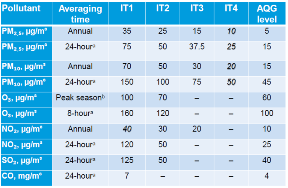
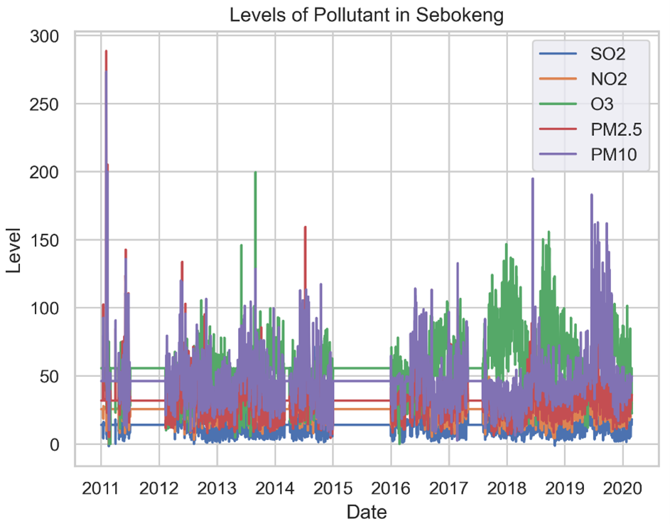
From the original dataset, the general concentrations of pollutants from highest to lowest were O₃, PM10, PM2.5, NO₂, and SO₂. The mean measurements over a 9-year period for all the pollutants are significantly higher than the recommended levels proposed by the Global Air Quality Guidelines (AQG), which were released by the World Health Organization (WHO) in September 2021 (Figure 1) (Garland et al., 2021). Comparing Sebokeng’s average levels of pollutants, the mode for SO₂ (3.45 μg/m3) sits between the WHO Interim Target (IT) 3 and the AQG, the mean for NO₂ (25.35 μg/m3) is between the annual IT-2 and IT-3; PM2.5 (31.67 μg/m3) is between IT-1 and IT-2; and PM10 (46.37 μg/m3) is between IT-2 and IT-3.

An analysis of the plot graph in Figure 2 shows PM10 as an outlier during January 2011, February 2017, April 2018, and from June to September 2019. Similarly, PM2.5 was an outlier in January 2011 and June 2014.

The observed correlations between the pollutant were generally weak. The strongest positive association was between PM2.5 and PM10 (0.71), while the strongest negative correlation was found between O₃ and NO₂. The strong correlation between PM2.5 and PM10 suggests that they may have similar emission sources (Zhou et al., 2016). According to Muyemeki et al. (2021), the positive correlation between PM2.5 and PM10 emanates from dust-related contributions (over 60%) and secondary aerosols (11%) from predominantly domestic coal burning.

Assessing Missing Data

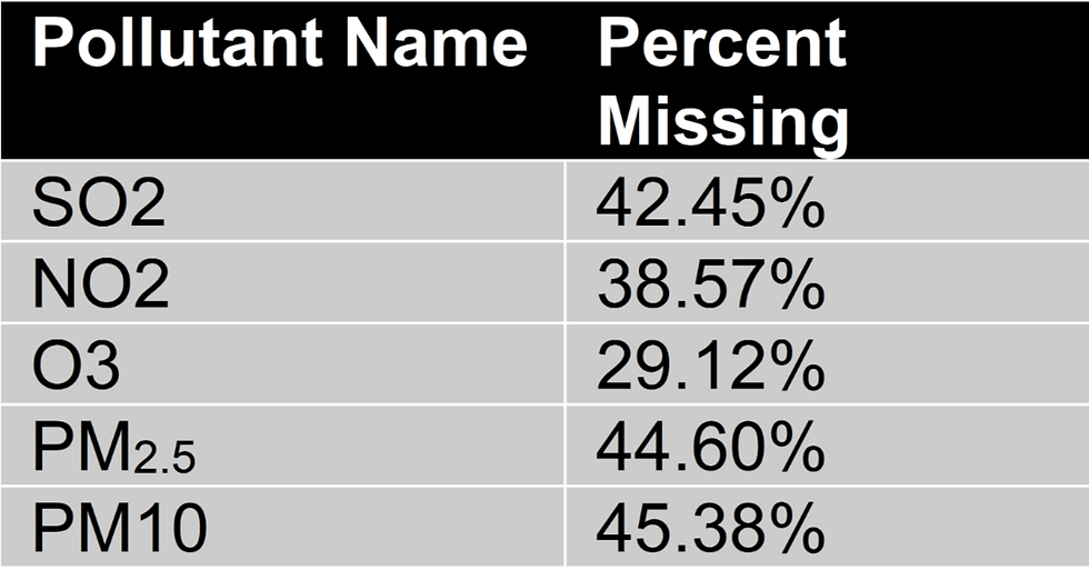
Table 2 shows the percentages of missing data were observed for each pollutant:

Table 2: Percentage of Missing Data

Data was notably missing during the following periods:

• May 2011 to January 2012

• March 2014

• January 2015 to January 2016 (the largest period of missing data)

• May 2017 to July 2017

Justification for Using MICE Imputation

Given the significant amounts of missing data, we assumed it to be missing at random (MAR). Multivariate Imputation by Chained-Equations (MICE) was chosen as it can estimate missing values based on the relationships between multiple variables. This method addresses gaps by iteratively generating predicted values for the missing entries (Kunal, 2024). During each cycle, the missing values for one variable are estimated using the information from the other variables. The process is repeated multiple times until the results stabilize, indicating that convergence has been achieved (Kunal, 2024).

Time-Series of Imputed Data vs. Raw Data

Figure 4 shows the plot graph of the imputed dataset of pollutant levels. As seen, this imputation only assists in identifying the comparative levels of the pollutants over the nine years.

Conclusion

This analysis reveals high pollutant levels in Sebokeng, with concentrations often exceeding WHO guidelines. PM10 and PM2.5 frequently appeared as outliers, likely influenced by industrial activity or seasonal factors, and showed a strong correlation, suggesting shared sources. Missing data posed a challenge, with some pollutants having over 40% of their data absent. Applying MICE imputation addressed these gaps, providing a more complete view of trends and relationships. Strengthening monitoring efforts and ensuring consistent data collection will improve future analyses and support better air quality management in the area.

---

Code

import pandas as pd
import matplotlib.pyplot as plt 
import numpy as np
from sklearn.experimental import enable_iterative_imputer
from sklearn.impute import IterativeImputer

# Load the dataset and create a copy of it
data = pd.read_excel("C:\\Users\\svuku\\Downloads\\Lab Assesment 1.xlsx", sheet_name="lecture 2_data")
data_copy = data.copy()

# Identify Missing Data and Create a Mask for them
missing_data = data.isnull().sum()
print(missing_data)

# Create a mask for missing values
missing_mask = data.isnull()  # This creates a boolean mask where True indicates missing values

# Initialize MICE IterativeImputer
imputer = IterativeImputer(max_iter=10, random_state=0)

# Fit the Imputer on the data and transform it to obtain the imputed values
imputed_values = imputer.fit_transform(data_copy)

# Correctly assign the imputed values to the missing locations
data_copy[:] = np.where(missing_mask, imputed_values, data_copy)

data_copy.to_excel("C:\\Users\\svuku\\Downloads\\Imputed_Dataset.xlsx", index=False)

---

References

Garland, R., Wernecke, B., Feig, G., & Langerman, K. (2021). The new WHO Global Air Quality Guidelines: What do they mean for South Africa? Clean Air Journal, 31(2). https://doi.org/10.17159/caj/2020/31/2.12915

Hadeed, S. J., O'Rourke, M. K., Burgess, J. L., Harris, R. B., & Canales, R. A. (2020). Imputation methods for addressing missing data in short-term monitoring of air pollutants. The Science of the total environment, 730, 139140. https://doi.org/10.1016/j.scitotenv.2020.139140

Kunal. (2024, January 16). Multivariate Imputation by Chained-Equations (MICE). Medium. https://medium.com/@kunalshrm175/multivariate-imputation-by-chained-equations-mice-2d3efb063434

‌

Muyemeki, L., Burger, R., Piketh, S. J., Beukes, J. P., & Van Zyl, P. G. (2021). Source apportionment of ambient PM10-25 and PM2. 5 for the Vaal Triangle, South Africa. South African Journal of Science, 117(5-6), 1-11.

Zhou, X., Cao, Z., Ma, Y., Wang, L., Wu, R., & Wang, W. (2016). Concentrations, correlations and chemical species of PM2.5/PM10 based on published data in China: Potential implications for the revised particulate standard. Chemosphere, 144, 518-526. https://doi.org/https://doi.org/10.1016/j.chemosphere.2015.09.003